\gdef\R{\mathbb{R}} \gdef\delim#1#2#3{#1 #2 #3} \gdef\p#1{({#1})} \gdef\abs#1{\lvert{#1}\rvert} \gdef\argmin{\mathop{\operatorname{arg\,min}}\limits} \gdef\e{\mathrm{e}}
Approximation theory
\gdef\e{\mathrm{e}} \gdef\delim#1#2#3{\mathopen{}\mathclose{\left#1 #2 \right#3}} \gdef\p#1{\delim({#1})} \gdef\abs#1{\delim\vert{#1}\vert}
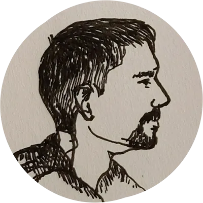
Consider this simple function:
f(x) = \e^{-x^2}
you may recognize it from such hits as the normal distribution and gaussian blur. It has loads of applications, so we want to use it!
But what if we are in strange new lands where we only have basic math operations? Or a direct implementation doesn't have quite the performance we are looking for?
Taylor series
The first thing a calculus 101 graduate does is compute the Taylor series. After a moment with pen and paper the first ten terms turn out to be:
p(x) = 1 - 2 ⋅ x^2 + 12 ⋅ x^4 - 120 ⋅ x^6 + 1680 ⋅ x^8
Every other term turned out zero! That feels a bit wasteful. It must have something to do with odd and even functions.
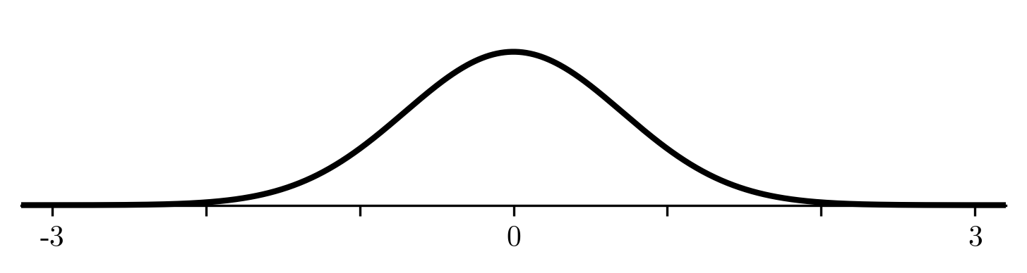
Now we have a nice polynomial that we can compute using basic operations. We can even trade off accuracy for performance by using fewer terms. Let's see what it looks like with the 3, 5, 7 and 9th Taylor polynomial (dashed line is the target function):
That's... terrible. We'll never get our function implemented this way. Time to think.
Minimize the maximum error
So what is the goal? We want to find a simple-to-implement function p(x) that best approximates our target function f on the domain of interest [-3, 3].
What makes an approximation better or worse? We want to give some hard guarantee like "this approximation is accurate to 12 decimals". For that, we need to consider the worst case behaviour, where the error is largest. This is maximum of \abs{f(x) - p(x)} in the domain. We want the p(x) that minimizes this value. In math-speak, we want:
\argmin_{p} \max_{x ∈ [a, b]} \abs{f(x) - p(x)}
This is the minimax approximation. It is different from the more common least squares approximation. Minimax is much harder to solve which is why least squares is more popular, but for use cases like approximation you really need the robust guarantees that you can only get from minimax. In this post I'll show you how to solve these minimax problems by building up to it.
Before we go any further, often the first thing you do when approximating a function is exploit its symmetries to reduce the range. For example, our target function is symmetrical around the vertical axis: f(-x) = f(x). We can use this to reduce the domain to [0, 3]:
def p(x):
assert -3 <= x and x <= 3
x = abs()
# ... rest of the function, now with x in [0, 3]Now we just need to implement p(x) on [0,3] using only basic operations.
Polynomial interpolation
With the basic operations addition and multiplication we can only construct polynomials. (If we also have division we can do rational functions, more on that later.) For now we want polynomials that we can implement using few operations. A pretty good way to implement polynomials is Horner's method (it is a common misconception that Horner's method is optimal, but this is a subject for another blog post.) Using Horner's method, the number of operations is proportional to the number of terms in the polynomial. Let's start with a five term polynomial:
p(x) = p_0 + p_1 ⋅ x + p_2 ⋅ x^2 + p_3 ⋅ x^3 + p_4 ⋅ x^4
It has five parameters p_i that we need to pick. One way to do this is by picking five points (x_i, y_i) on the target function and insisting that the polynomial goes through those points. Let's pick n=5 points evenly spaced over the domain [a, b]=[0,3]:
\begin{aligned} x_i &= a + \frac{i}{n - 1}\p{b-a} &&& y_i &= f(x_i) \end{aligned}
This results in five equations p(x_i) = y_i. Fully expanded, each one looks like
p_0 + p_1 ⋅ x_i + p_2 ⋅ x_i^2 + p_3 ⋅ x_i^3 + p_4 ⋅ x_i^4 = y_i
We know the (x_i, y_i)'s and want to solve for the p_i's. We can compute all the powers of x_i and we end up with p_i's multiplied by constants; a system of linear equations. We can write this as a matrix:
\def\arraystretch{1.3} \begin{bmatrix} 1 & x_0 & x_0^2 & x_0^3 & x_0^4 \\ 1 & x_1 & x_1^2 & x_1^3 & x_1^4 \\ 1 & x_2 & x_2^2 & x_2^3 & x_2^4 \\ 1 & x_3 & x_3^2 & x_3^3 & x_3^4 \\ 1 & x_4 & x_4^2 & x_4^3 & x_4^4 \end{bmatrix} \cdot \begin{bmatrix} p_0 \\ p_1 \\ p_2 \\ p_3 \\ p_4 \end{bmatrix} = \begin{bmatrix} y_0 \\ y_1 \\ y_2 \\ y_3 \\ y_4 \end{bmatrix}
This kind of matrix is called a Vandermonde matrix. We can solve it using basic linear algebra to get our p_i's. In this case
p_i = \small\begin{bmatrix} 1.0000 & -0.1493 & -0.9330 & 0.5560 & -0.0885 \end{bmatrix}
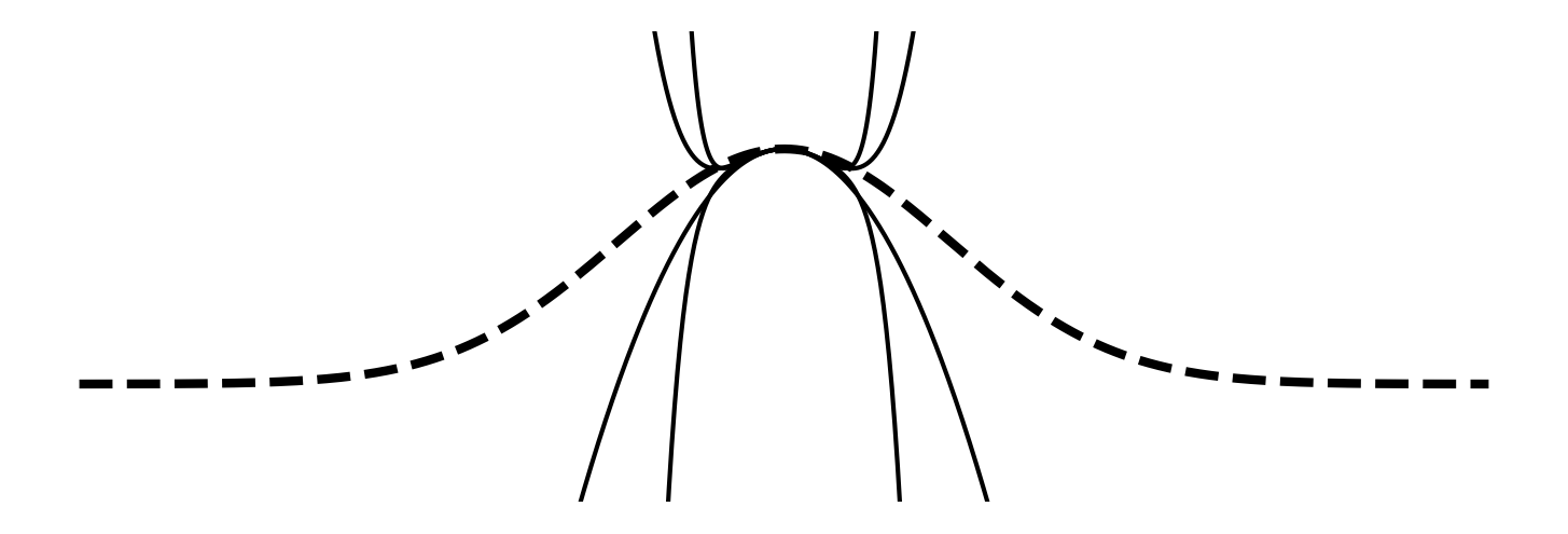
The solution polynomial we found looks like
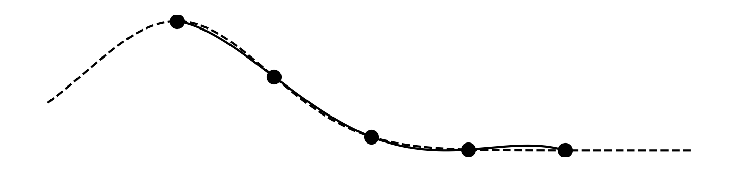
That is much better than any of our Taylor polynomials, and we used only five terms instead of ten! In fact, it's already hard to see the error, so let's zoom in on the error p(x) - f(x):
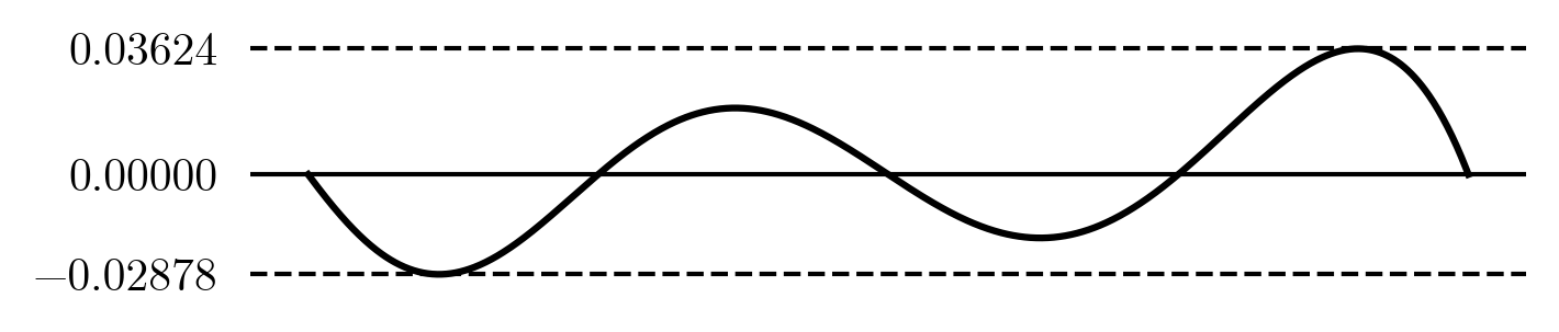
It's nicely meandering back and forth around zero, crossing zero exactly where we picked the x_i values. It has a maximum error less than 0.037.
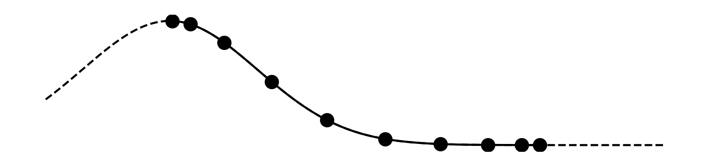
What if we use ten terms? We can re-do all the above with n=10 points and we get:
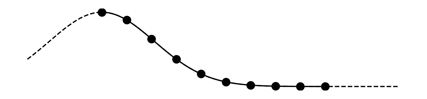
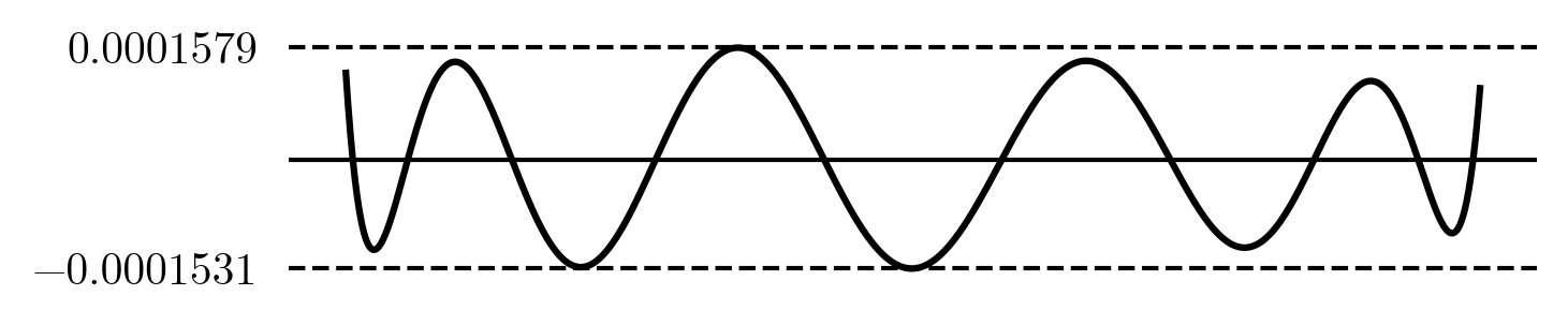
The approximation now looks perfect! We need to look at the error to see what is going on:
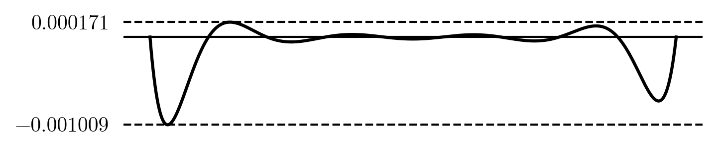
The maximum error is now nearly 0.001, almost 3 decimals of precision! Notice how the largest error is again at the ends. This gets worse as we add more terms and is an example of Runge's phenomenon. Let's fix that!
Chebyshev nodes
Runge's phenomenon happens on equaly spaced interpolations. To counter it we need to move the points more towards the edges. Intuitively this forces the polynomial to learn more about the edges and be more accurate there. A special set of points called Chebyshev nodes does this. On the domain [a, b] they are defined as
\begin{aligned} x_i &= \frac{a+b}{2} + \frac{b-a}{2} \cos\p{\frac{2 ⋅i + 1}{2 ⋅ n} ⋅ π} &&& y_i &= f(x_i) \end{aligned}
Using these points, the five term interpolation looks like
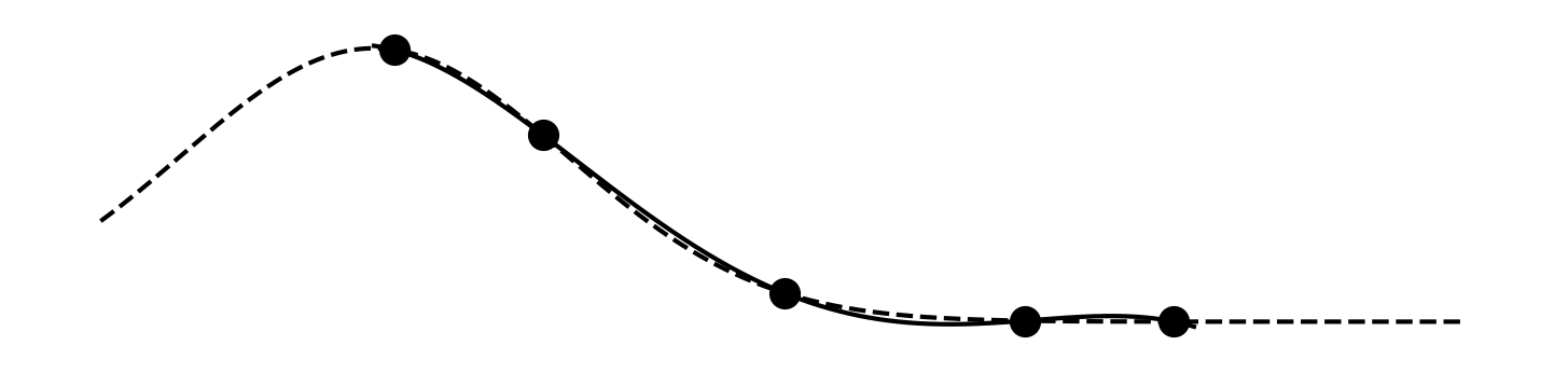
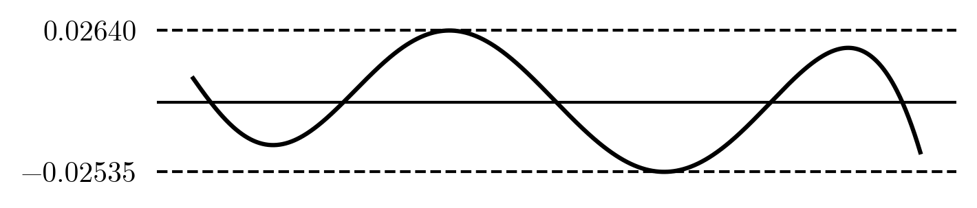
The maximum error reduced slightly and no longer happens at the ends. With Chebyshev nodes the ten term interpolation looks like
The error is about 1.5\cdot10^{-4} that is nearly four accurate digits, a 10x improvement over the previous equispaced version! There is also no sign of Runge's phenomenon anymore.
The equioscilation theorem
If you look at the last error plot you'll notice how the error wobbles smoothly and uniformly from negative to positive, instead of having large peaks like before. This apparently results in a lower overall error. It makes intuitive sense: by spreading the error evenly over all places, it doesn't pile up in a big peak and we reduce the maximum error.
This is actually a profound fact called the equioscillation theorem. In plain words a n-term polynomial is the best possible approximation if and only if its error goes back and forth at least n + 1 times, each time hitting the maximum error.
We can find this optimum manually: by moving the points x_i around we can reduce the error in an area by moving the points a little closer there, or moving them away from areas where the error is very small. If we keep doing this we will end up with all the 'error' evenly spread out. Starting with the five term Chebyshev solution, after a lot of manual fiddling with values we find a 'tuned' set of x_i that gives a decently flat error:
x_i = \small \begin{bmatrix} 0.11 & 0.72 & 1.51 & 2.34 & 2.92 \end{bmatrix}
But this is a lot of work, let's automate it.
Remez algorithm
The hero of this story is Е.Я́. Ре́мез (Remez) from Kyiv University. He's known for the Remez algorithm that finds the optimal polynomial automatically. The algorithm works backwards from the equioscillation theorem: assume that our polynomial p(x) satisfies the equioscillation theorem, then there is a set of points x_i such that
p(x_i) = f(x_i) \pm e
where e is the maximum error and \pm alternates signs. This is the first great insight: instead of trying to interpolate the function perfectly, we interpolate it with error included. This way we control the error and can place it optimally. The points x_i are the n+2 peaks where we want the maximum error to manifest. Writing this out for a five term polynomial we get equations
p_0 + p_1 ⋅ x_i + p_2 ⋅ x_i^2 + p_3 ⋅ x_i^3 + p_4 ⋅ x_i^4 \pm e = y_i
If we knew the values x_i this would again be a linear equation with unknowns p_i. In fact, we have n+1 equations, so we can use the extra equation to also solve for the maximum error e. But we don't know the x_i coordinates of the error maxima. The second great insight Remez had was that: if you start with approximate values x_i you will get better ones. Cool! So let's take the x_i from our five term Chebyshev. That is, we find the x coordinates of all the peaks in the error:
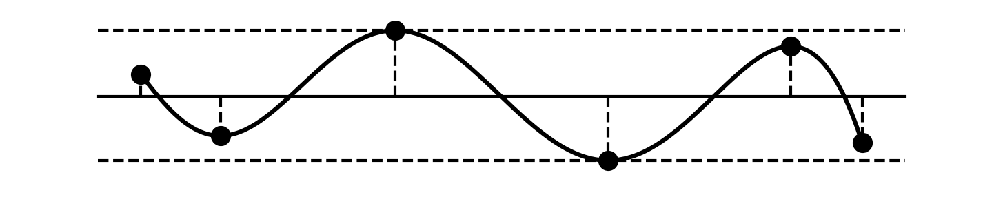
With these x_i we can write our equations as a linear algebra problem
\def\arraystretch{1.3} \begin{bmatrix} 1 & x_0 & x_0^2 & x_0^3 & x_0^4 & +1 \\ 1 & x_1 & x_1^2 & x_1^3 & x_1^4 & -1 \\ 1 & x_2 & x_2^2 & x_2^3 & x_2^4 & +1 \\ 1 & x_3 & x_3^2 & x_3^3 & x_3^4 & -1 \\ 1 & x_4 & x_4^2 & x_4^3 & x_4^4 & +1 \\ 1 & x_5 & x_5^2 & x_5^3 & x_5^4 & -1 \\ \end{bmatrix} \cdot \begin{bmatrix} c_0 \\ c_1 \\ c_2 \\ c_3 \\ c_4 \\ e \end{bmatrix} = \begin{bmatrix} y_0 \\ y_1 \\ y_2 \\ y_3 \\ y_4 \\ y_5 \end{bmatrix}
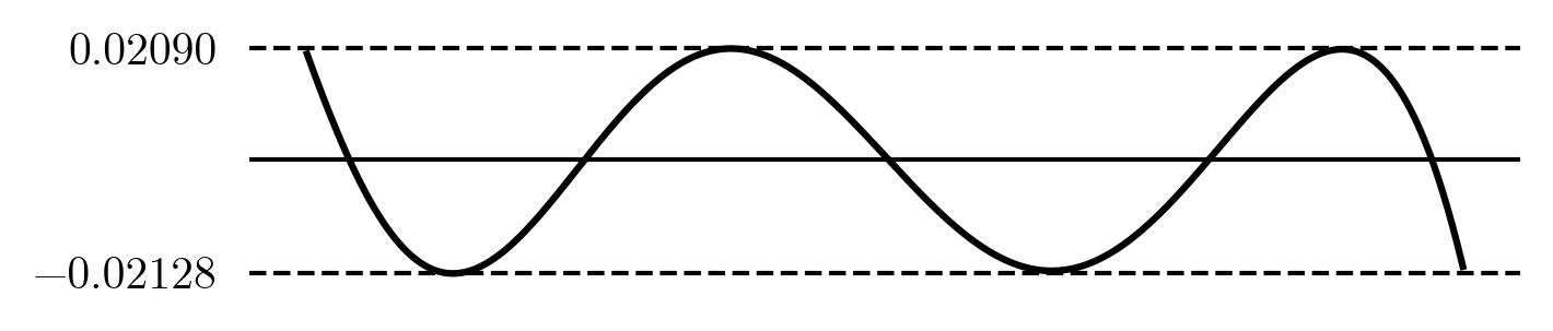
This gets us values for p_i and e=0.0209. Neat! Let's plot the error for our new five term polynomial:

It is indeed looking more optimal than the Chebyshev we started with; the errors all look close to the same height! The actual error is 0.0212, that is a 20\% improvement. Note that the computed error e does not match the actual error, this is due to our x_i's being inaccurate. The solution is already better than our hand-tuned one, but it's not perfect yet as there are still slight difference in the peak heights.
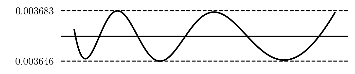
Remez is an iterative method. We repeat the same process, this time picking x_i's from the error peaks of the polynomial we just found. We get a new set of p_i's and e = 0.0208. The actual error is also 0.0208. This is a sign that the algorithm is converging on the optimal polynomial. Doing more iterations doesn't really change the result much, Remez converges pretty fast. This is what we get:
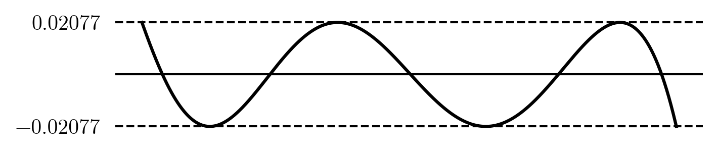
This is what perfection looks like! It goes back and forth six times, hitting the maximum error each time. By the equioscillation theorem, this is the best possible approximation with a five term polynomial. It is however only a \small 21\% reduction of the error compared to Chebyshev. Generally Chebyshev polynomials are already close to optimal. This will change when we get to rational approximations in a moment.
When using Remez, it can sometimes happen that the error has more than n+1 peaks. If this happens a good strategy is to take a subsequence of n+1 peaks such that their signs alternate and the smallest one is as large as possible.
Rational approximation
What if we can do addition, multiplication, and also division? Every function we can construct with these will be a rational function. They are not nearly as well known a the polynomials and this needs to change! They are not very difficult as every rational function h(x) can be written as a fraction of two polynomials
h(x) = \frac{p(x)}{q(x)} = \frac{p_0 + p_1 ⋅x + p_2 ⋅x^2}{q_0 + q_1 ⋅ x + q_2 ⋅ x^2 + q_3 ⋅ x^3}
We now need to pick the number of terms for both p(x) and q(x). Let's call the above the \small (3,4)-term rational function. This formula looks like it has seven parameters, but it's really one less: just like how fractions can be reduced, for example \frac{9}{12} = \frac{3}{4}, the rational functions can also be 'reduced' by dividing out a common factor. For example we can divide out q_0, effectively setting q_0 = 1. The other parameters can still take any value (though they will be different by a factor \frac{1}{q_0}. We could have picked any parameter and fix it to any non-zero value, but q_0=1 makes the math easier. Another common convention is to set q_{n-1} = 1, which saves a single multiplication when evaluating. It is easy to convert between the two.
Let's create a five-parameter rational approximation to compare with the five-parameter polynomial from before. Specifically let's look at a \small (3,3)-term rational function:
h(x) = \frac{p(x)}{q(x)} = \frac{p_0 + p_1 ⋅x + p_2 ⋅x^2}{1 + q_1 ⋅ x + q_2 ⋅ x^2}
Like before, to solve for p_i and q_i we interpolate through points (x_i, y_i). This time a bit more algebra is required:
$$ \begin{aligned} h(x_i) &= \frac{p(x_i)}{q(x_i)} = y_i &\Rightarrow&& p(x_i) &= y_i ⋅ q(x_i) &\Rightarrow \[0.5em] \end{aligned}
\begin{aligned} &p_0 + p_1 ⋅x_i + p_2 ⋅x_i^2 = y_i ⋅\p{1 + q_1 ⋅ x + q_2 ⋅ x^2} \Rightarrow\[0.7em] &p_0 + p_1 ⋅x_i + p_2 ⋅x_i^2 - q_1 ⋅ y_i ⋅ x_i - q_2 ⋅ y_i ⋅ x_i^2 = y_i \end{aligned} $$
Since x_i and y_i are constant, this is again linear and we can solve for p_i and q_i. The linear system is
\def\arraystretch{1.3} \begin{bmatrix} 1 & x_0 & x_0^2 & - y_0 ⋅ x_0 & - y_0 ⋅ x_0^2 \\ 1 & x_1 & x_1^2 & - y_1 ⋅ x_1 & - y_1 ⋅ x_1^2 \\ 1 & x_2 & x_2^2 & - y_2 ⋅ x_2 & - y_2 ⋅ x_2^2 \\ 1 & x_3 & x_3^2 & - y_3 ⋅ x_3 & - y_3 ⋅ x_3^2 \\ 1 & x_4 & x_4^2 & - y_4 ⋅ x_4 & - y_4 ⋅ x_4^2 \\ \end{bmatrix} \cdot \begin{bmatrix} p_0 \\ p_1 \\ p_2 \\ q_0 \\ q_1 \end{bmatrix} = \begin{bmatrix} y_0 \\ y_1 \\ y_2 \\ y_3 \\ y_4 \\ \end{bmatrix}
Using the same five Chebyshev points (x_i, y_i) as before we find the solution
\begin{aligned} p_i &= \small\begin{bmatrix} 0.99524975 & -0.72539761 & 0.13181353 \end{bmatrix} \\ q_i &= \small\begin{bmatrix} 1.00000000 & -0.77962832 & 0.93440655 \end{bmatrix} \end{aligned}
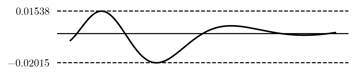
The maximum error is now \small 0.02015, this is even better than the optimal five-term polynomial we found. It does look like all the error is on the left now. Can we move points around and get a better result like before? Let's manually move the x_i's around again. After some fiddling and nudging the x_i's we find a set that works well:
x_i = \small \begin{bmatrix} 0.29 & 0.73 & 1.28 & 1.99 & 2.82 \end{bmatrix}
We got the error to drop $\small 81$% and nearly got a whole extra digit of precision! So clearly rational functions are promising and fine-tuning them has a big impact. Notice that as it got better, it also starts to look more like a nice equioscillation error. It is a little know fact (not even Wikipedia mentions it) that the equioscillation theorem also applies to rational functions!
You may be wondering why we picked a \small (3,3)-term rational function, and not one of the other five parameter options. The \small (5,1)-term rational function is simply the five term polynomial we saw before. But let's look at the \small (4,2)-term one. We can solve the equations as before and get the solution:
\begin{aligned} p_i &= \small\begin{bmatrix} 1.04506339 & -1.58632468 & 0.74871783 & -0.11232492 \end{bmatrix} \\ q_i &= \small\begin{bmatrix} 1.00000000 & -0.84949604 \end{bmatrix} \end{aligned}
But when we plot h(x) = p(x)/q(x) function we get
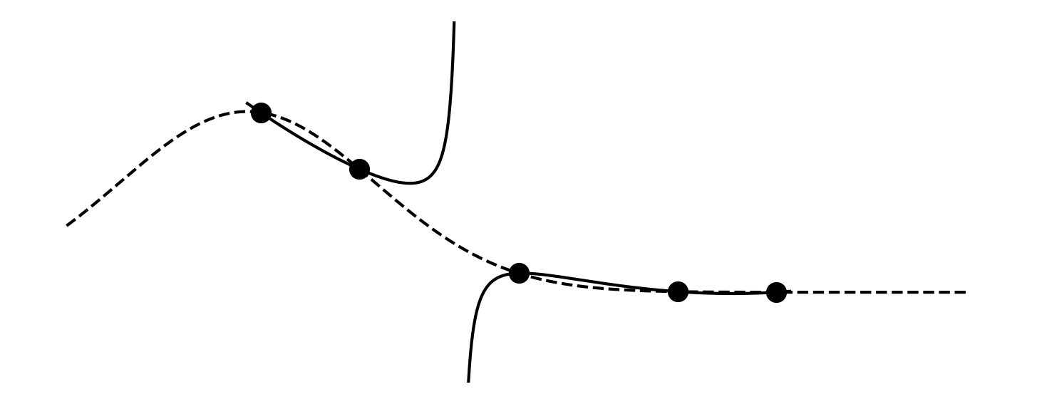
Whoops! That does not look good! It goes through the five points alright, but what happens between the second and third point? A bit of debugging and you find that at x = q_1^{-1} ≈ 1.18 we have q(x) = 0 and thus a division by zero. We can not use solutions where q(x) has a zero in the domain. It turns out some combinations of (n,m)-terms simply don't work. A good strategy is to try all combinations and pick the one that gives the best result. For five terms \small (3,3) is optimal.
Rational-Remez
For rational functions the Cehbyshev solution is good, but fine-tuning has a big impact. Let's try to optimize this process with Remez algorithm again. We start the same by working backwards from the goal. The algebra is a bit more complex now, but we get
\begin{aligned} h(x_i) &= y_i \pm e &\Rightarrow&& \frac{p(x_i)}{q(x_i)} &= y_i \pm e &\Rightarrow&& p(x_i) &= \p{y_i \pm e} ⋅ q(x_i) \\[1em] p_0 + p_1 ⋅ x_i + p_2 ⋅x_i^2 &= \p{y_i \pm e} ⋅ \p{1 + q_1 ⋅ x_i + q_2 ⋅ x_i^2} \\[1em] p_0 + p_1 ⋅ x_i + p_2 ⋅x_i^2 - q_1 ⋅ \p{y_i \pm e} ⋅ x_i - q_2 ⋅ \p{y_i \pm e} ⋅ x_i^2 \mp e &= y_i \end{aligned}
Hmm. We now have e terms added to our y_i's. We can't solve this like before where we guess x_i and y_i and solve for p_i, q_i, and e. Fortunately, we can also guess e from an approximate solution. We can still solve for the final e term, this will come in handy in a moment. Writing this out in linear algebra again
\def\arraystretch{1.3} \begin{bmatrix} 1 & x_0 & x_0^2 & - \p{y_0 + e} ⋅ x_0 & - \p{y_0 + e} ⋅ x_0^2 & -1 \\ 1 & x_1 & x_1^2 & - \p{y_1 - e} ⋅ x_0 & - \p{y_1 - e} ⋅ x_1^2 & +1 \\ 1 & x_2 & x_2^2 & - \p{y_2 + e} ⋅ x_0 & - \p{y_2 + e} ⋅ x_2^2 & -1 \\ 1 & x_3 & x_3^2 & - \p{y_3 - e} ⋅ x_0 & - \p{y_3 - e} ⋅ x_3^2 & +1 \\ 1 & x_4 & x_4^2 & - \p{y_4 + e} ⋅ x_0 & - \p{y_4 + e} ⋅ x_4^2 & -1 \\ 1 & x_5 & x_5^2 & - \p{y_5 + e} ⋅ x_0 & - \p{y_5 + e} ⋅ x_5^2 & +1 \\ \end{bmatrix} \cdot \begin{bmatrix} p_0 \\ p_1 \\ p_2 \\ q_1 \\ q_2 \\ e' \end{bmatrix} = \begin{bmatrix} y_0 \\ y_1 \\ y_2 \\ y_3 \\ y_4 \\ y_5 \end{bmatrix}
Like before, we can start the Remez iteration with an initial Chebyshev solution. Take the x_i's from the error peaks, take y_i = f(x_i), and this time we also guess e to be the maximum error from the initial solution. This will give us an output error e' that is likely different from our guessed e. The first step is to make these two equal by picking a better guess for e. There are different methods for doing this, but what worked well for me is taking the mean of the guess and computed value, i.e. the new guess for e is \frac{e + e'}{2}. If we iterate this process a couple of times e and e' will converge. This means we found a solution to our non-linear problem. We then take the resulting function, and like before update our guesses for the x_i's. We repeat this whole process a few times until the Rational-Remez converges, each time solving for e first before updating the x_i's. The final result has an error that looks like
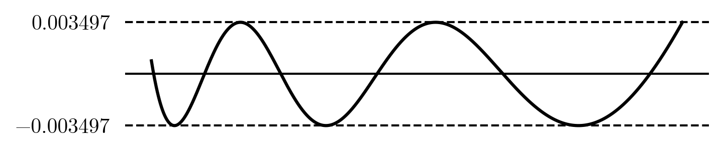
This is the best possible \small (3,3)-term rational function. It has a \small 6 times smaller error than the Chebyshev rational and \small 8 times smaller than the Chebyshev polynomial.
Method comparison
I picked five parameters because it shows how things work while still allowing readable explicit formulas. The pattern should be clear and can be generalized to any number of parameters.
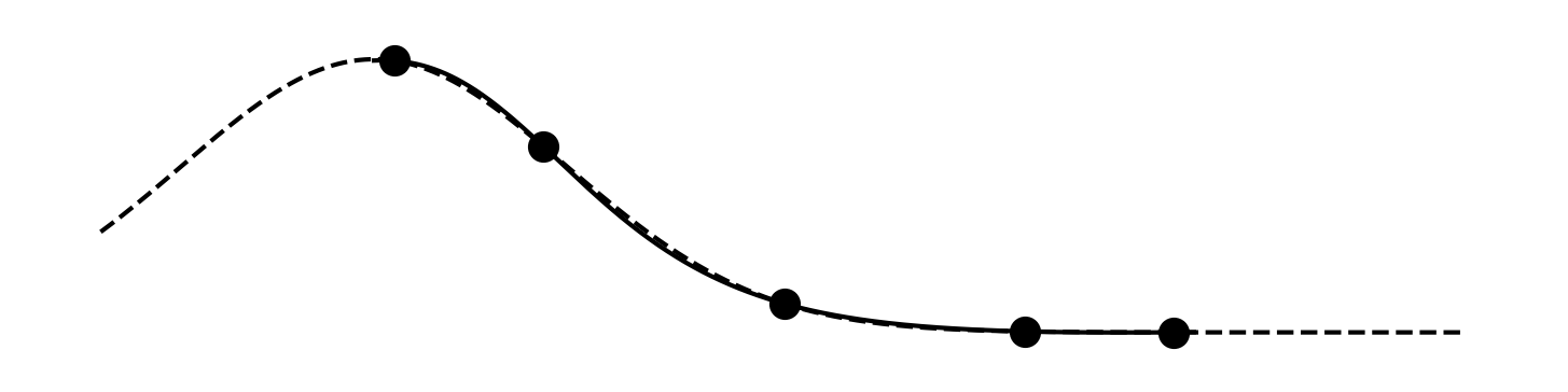
From equispaced to Remez-Rational, we now have five progressively more sophisticated approximation methods. To compare them, we can plot how many decimal digits of accuracy they give for increasing numbers of parameters:
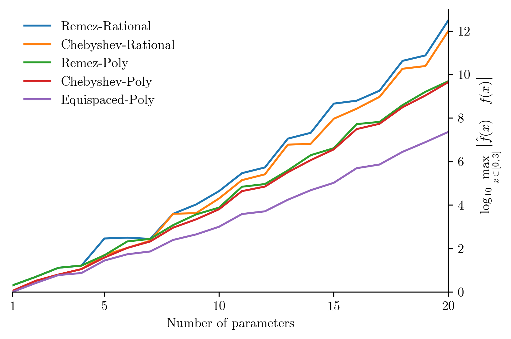
In this figure we can see that Chebyshev polynomial approximations are significantly better than equispaced ones and in fact they are almost as good as the optimal Remez polynomials. This validates the common wisdom that for polynomials Chebyshev is good enough and Remez is not worth the complexity.
What we see here is that rational functions have a significant advantage over plain polynomials. Here Chebyshev points alone leave some accuracy on the table and optimizing using the rational Remez algorithm pays of.
All of the above assumes we are working with real numbers \R but in reality computers have limited precision. When finding and evaluation approximation functions it is convenient to use an arbitrary precision library like mpfr or mpmath. Then crank up the precision to much higher than your target. That way we don't have to worry about it. You can find a Jupyter notebook implementation here.
Key takeaways
- 🌟 Almost any function can be approximated efficiently.
- 👉 First use knowledge of your function to reduce the domain.
- 🚫 Don't use Taylor series or equispaced points.
- ✅ Use Chebyshev approximation if you need a polynomial.
- 🚀 Rational functions can offer a significant improvement.
- 🤓 Remez on rational functions is difficult, but offers an improvement.
- 👉 Use a high-precision arithmetic library to find approximations.
What's next
Once you have found an approximation you are happy with, the next step is to implement it. This is where we have to leave arbitrary precision arithmetic behind and instead use integer, fixed-point or floating-point math. This introduces new errors that must be mitigated or accounted for. “Evaluating polynomials efficiently and accurately” is a topic for a future post.
References
- L.N. Trefethen (2019). “Approximation Theory and Approximation Practice.” available online
- T.A. Driscoll, N. Hale, and L.N. Trefethen, editors (2014) "Chebfun Guide” website
- ARM Limited (2019). Remez routine source code. github
- J.J. O'Connor and E.F. Robertson (2018). “Evgeny Yakovlevich Remez” link
- N. Agrawal et al. (2021). “Boost C++ v. 1.78.0: The Remez Method.” link
- C.B. Dunham (1975). “Convergence of the Fraser-Hart Algorithm for Rational Chebyshev Approximation.” pdf
Big thank you to Transmissions XI for provoking me to write this and great feedback on early versions of this article.