\gdef\R{\mathbb{R}} \gdef\delim#1#2#3{\mathopen{}\mathclose{\left#1 #2 \right#3}} \gdef\p#1{({#1})} \gdef\dummyarg{\operatorname{-}} \gdef\d{\operatorname{d}\!} \gdef\Pr#1{\operatorname{Pr}\p{#1}} \gdef\E#1{\operatorname{E}[{#1}]} \gdef\Es#1{\operatorname{E}_{#1}} \gdef\Var#1{\operatorname{Var}\p{#1}} \gdef\DKL#1#2{\operatorname{D_{KL}}({#1} \Vert {#2})} \gdef\argmax{\mathop{\operatorname{arg\,max}}\limits}
Exploitation: Entropy & Utility
Given some probability distribution on future returns on a collection of assets, what is our best strategy for exploiting this knowledge?
To do. When is it better to wait because future information will improve our strategy?
Goal
What to optimize for?
Von Neumann–Morgenstern utility theorem
Given a set of possible strategies S and stochastic portfolio value V_i(s) for strategy s at time i the Kelly goal is to maximize the expected geometric growth rate:
\max_{s ∈ S} \E{ \lim_{n → ∞} \frac{1}{n} \ln \frac{V_n(s)}{V_0} }
For convenience we define the exponential rate of growth as G_n(s) = \frac{1}{n} \ln \frac{V_n(s)}{V_0} and G_∞ = \lim_{n → ∞} G_n, the goal then becomes \max_{s ∈ S} \E{G_∞(s)}
The Kelly strategy has several nice properties:
- The maximized expected geometric growth rate equals the information entropy.
- For any other essentially different strategy s', we have \lim_{n → ∞} \frac{V_n(s')}{V_n(s)} → 0 almost surely.
- For any value the X the Kelly strategy minimizes the expected time to reach this goal.
The set of strategies S is deliberately left unspecified. It can include strategies that uses previous realizations V_i(s) to inform decisions and it can make use of external information. In many examples the strategy is a fixed allocation f \in \R^n, \sum_i f_i = 1.
Side quests
The common criticism on the Kelly strategy is that it has too much downside risk. While it maximizes long-term growth, it is willing to endure substantial short-term losses to get there. In repeated betting examples a reduction in risk taken (in the form of more allocation to a risk-free asset) leads to a substantial decrease in downside risk, while preserving much of the growth.
The Kelly strategy is also somewhat sensitive to errors. If the model used is optimisitc, it will lead to taking to much risk which increases the probability of ruin.
Both these reasons suggest lowering the risk. Thorp promotes a strategy called fractional Kelly where only a fraction c of the Kelly optimum is betted. (Q: How does this generalize to portfolio's with a risk-free asset?)
Proebstring's paradox
https://en.wikipedia.org/wiki/Proebsting%27s_paradox
https://statweb.stanford.edu/~lpekelis/papers/3_12_proebsting_pekelis.pdf
The discrete problem
The story starts with Kelly betting. In this simplified version of the problem there is a repeated opportunity to place a bet. In the simplest case where the bet results in a win of b with probability p, and nothing on loss, the optimal amount to bet is:
p - \frac{1 - p}{b}
The method has been generalized and developed further by E.O. Thorp. Recently the discussion evolved to include probability distributions changing on new insights.
-
https://en.wikipedia.org/wiki/Proebsting%27s_paradox
-
J.L. Kelly (1956). "A New Interpretation of Information Rate" https://www.princeton.edu/~wbialek/rome/refs/kelly_56.pdf
-
E.O. Thorp (2007). "The Kelly Criterion in Blackjack sports betting and the stock market" https://wayback.archive-it.org/all/20090320125959/http://www.edwardothorp.com/sitebuildercontent/sitebuilderfiles/KellyCriterion2007.pdf
-
Vasily Nekrasov (2014). "Kelly criterion for multivariate portfolios:a model-free approach" https://papers.ssrn.com/sol3/papers.cfm?abstract_id=2259133
The continuous problem
https://en.wikipedia.org/wiki/Merton%27s_portfolio_problem
Models
A simple way to model returns is as geometric Brownian motion. This is how it is modelled in the Black-Scholes equation for example.
To do. Solve for multi-asset GBM first, before looking into more complex models.
Extensions of this model have been developed under the heading of (Stochastic Volatility)[https://en.wikipedia.org/wiki/Stochastic_volatility] models.
References
- https://www.sportsbookreview.com/forum/handicapper-think-tank/29009-expected-value-vs-expected-growth-kelly-criterion-part-i.html#post250260
- https://www.sportsbookreview.com/forum/handicapper-think-tank/29841-maximizing-expected-growth-kelly-criterion-part-ii.html
- https://blog.alphatheory.com/2013/01/kelly-criterion-in-practice-grizzlyrock-capital-part-1.html
- https://blog.alphatheory.com/2013/01/kelly-criterion-in-practice-grizzlyrock-capital-part-2.html
Information Theory Recap
- C.E. Shannon (1948). "A Mathematical Theory of Communication"
Given a random variable X with discrete outcomes x_i, the entropy H(X) is
H(X) = - \sum_i P(x_i) \log_2 P(x_i)
The I(x_i) = -\log_2 P(x_i) term is the information content of outcome x_i and I is a new random variable derived from X such that H(X) = E(I).
H\p{X \mid Y} = - \sum_{i,j} p_{i,j} \log \frac{p_{i,j}}{p_j}
Mutual information I(X;Y) = I(Y;X) \ge 0
I(X;Y) = \sum_{x\in X} \sum_{y \in Y} p(x, y) \log_2 \frac{p(x,y)}{p(x) \cdot p(y)}
https://en.wikipedia.org/wiki/Mutual_information#/media/File:Figchannel2017ab.svg
Entropy
My all-time favorite paper is Shannon's "A Mathematical Theory of Communication". Available in PDF here.
The basic Shannon entropy
\gdef\H{\operatorname{H}} \gdef\I{\operatorname{I}}
\H(X) = - \sum_i \Pr{x_i} ⋅ \log \Pr{x_i}
This is the expected value \H(X) = \E{\I\p{X}} of the information content \I:
\I(x) = - \log \Pr{x}
Note. The information content of a random variable is itself a random variable.
Kelly
To do. I'm spending to much time on this. Kelly is nothing more than the observation that 1) log-utility maximizes growth, and 2) the maximal growth rate is related to the Shannon entropy.
Consider a simple bet X with two outcomes, with probability \frac 12 it pays out 2 times the inlay x and with probability \frac 12 it pays nothing. The expected payoff of this bet is \E{X} = x, so it is even money.
Suppose now we have access to perfect information on the outcomes and can always place the winning bet. The expected payoff is 2 x. For even odds this means we double our inlay each time. If we start with capital V_0 and place all of it in bets, after each bet we have capital V_i. Define the rate of growth G as
G ≜ \lim_{N → ∞} \frac 1N \log_2 \frac {V_N}{V_0}
With our perfect information V_i is almost surely 2^i ⋅ V_0, so the rate of growth is
\E{G} = \lim_{N → ∞} \frac 1N \log_2 \frac {2^N ⋅ V_0}{V_0} = \lim_{N → ∞} \frac 1N \log_2 2^N = 1
Consider now the case where our information is imperfect and with error probability p and probability of being correct q = 1 - p. If we continue betting all our capital on the predicted outcome each time the expected capital is
\E{V_N} = \p{2q}^N ⋅ V_0
However, the expected value here is deceiving, as one misplaced bet will lead to ruin. The probability of this happening after N bets is 1 - q^N and tends to one as N increases. So with probability q^N we have 2^N ⋅ V_0 and zero otherwise. (The commutation of \E{\dummyarg} with the limit is valid by the monotone convergence theorem).
\begin{aligned} \E{G} &= \E{\lim_{N → ∞} \frac 1N \log_2 \frac {V_N}{V_0}} \\ &= \lim_{N → ∞} \frac 1N \E{\log_2 \frac {V_N}{V_0}} \\ &= \lim_{N → ∞} \frac 1N \p{ q^N \p{\log_2 \frac {2^N ⋅ V_0}{V_0}} + \p{1 - q^N} \p{\log_2 \frac {0}{V_0}}} \\ &= \lim_{N → ∞} \frac 1N \p{ q^N \p{\log_2 2^N} + \p{1 - q^N} \p{\log_2 0}} \\ &= \lim_{N → ∞} \frac 1N \p{ q^N ⋅N + \p{1 - q^N} \p{-∞}} \\ &= -∞ \end{aligned}
So the expected growth is diverges to negative infinity. In fact this happens for all N ≥ 1. We can see that this happens whenever there is a finite chance of ruin. \E{G} strongly dislikes ruin.
Fractional bets
Instead of betting everything we now bet a fraction l of the capital each time. At bet N our capital is
V_N = (1 + l)^{W_N} ⋅ (1 - l)^{L_N} ⋅ V_0
Where W_N and L_N = N - W_N are random variables of the number of wins and losses in the N bets. W_N is binomially distributed with
\Pr{W_N = i} = \binom{N}{i} ⋅ q^i ⋅ p^{N - i}
Linear utility
The expected value can be computed using the binomial formula
\begin{aligned} \E{V_N} &= \sum_{i ∈ [0,N]} \binom{N}{i} ⋅ q^i ⋅ p^{N - i} ⋅ (1 + l)^i ⋅ (1 - l)^{N - i} ⋅ V_0 \\ &= V_0 ⋅ \sum_{i ∈ [0,N]} \binom{N}{i} ⋅ \p{q(1 + l)}^i ⋅ \p{p(1 - l)}^{N - i} \\ &= V_0 ⋅ \p{q(1 + l) + p(1 - l)}^N \\ &= \p{1 + (q-p)⋅l}^N ⋅ V_0 \\ \end{aligned}
Note that q-p = 2q -1 and we recover \p{2q}^N ⋅ V_0 for l =1. If we want to maximize \E{V_N}:
\begin{aligned} l_{\text{exp}} &≜ \argmax_l \ \E{V_N} \\ &= \argmax_l \ (q - p) l \\ &= \begin{cases} +∞ & q-p > 0 \\ -∞ & q-p < 0 \end{cases} \end{aligned}
The expectation maximizing strategy is basically to always take infinite leverage. Not exactly subtle. But at least it is sensible enough to bet against the information when q < \frac 12 and thus q-p < 0.
Log utility
Let's try maximizing growth.
\begin{aligned} \E{G} &= \E{\lim_{N → ∞} \frac 1N \log_2 \frac {V_N}{V_0}} \\ &= \E{\lim_{N → ∞} \frac 1N \log_2 \frac {(1 + l)^{W_N} ⋅ (1 - l)^{L_N} ⋅ V_0}{V_0}} \\ &= \E{\lim_{N → ∞} \frac 1N \log_2 \p{(1 + l)^{W_N} ⋅ (1 - l)^{L_N}}} \\ &= \E{\lim_{N → ∞} \p{ \frac{W_N}{N} \log_2 \p{1 + l} + \frac{L_N}{N} \log_2 \p{1 - l} } } \\ &= \E{ \p{\lim_{N → ∞} \frac{W_N}{N}} \log_2 \p{1 + l} + \p{\lim_{N → ∞} \frac{L_N}{N}} \log_2 \p{1 - l} } \\ &= q \log_2 \p{1 + l} + p \log_2 \p{1 - l} \\ \end{aligned}
To maximize we solve
0 = \frac{\d \E{G}}{\d l} = \frac{q}{\p{1 + l} \log 2} - \frac{p}{\p{1 - l} \log 2}
\frac{q}{\p{1 + l} \log 2} = \frac{p}{\p{1 - l} \log 2}
\frac{q}{1 + l} = \frac{p}{1 - l}
q \p{1 - l} = p \p{1 + l}
q - ql = p + p l
(q-p) = (q + p) l
l = \frac{q - p}{q + p} = q - p
For this l
\begin{aligned} \E{G} &= q \log_2 \p{1 + l} + p \log_2 \p{1 - l} \\ &= q \log_2 \p{1 + q - p} + p \log_2 \p{1 - q + p} \\ &= q \log_2 2q + p \log_2 2p \\ &= 1 + q \log_2 q + p \log_2 p \\ \end{aligned}
CRRA utility
\begin{aligned} \E{U(V_N)} &= \E{-V_N^{1 - α}} \\ &= - \E{\p{(1 + l)^{W_N} ⋅ (1 - l)^{L_N} ⋅ V_0}^{1-α}} \\ &= - V_0^{1-α} ⋅ \E{(1 + l)^{W_N ⋅ \p{1-α}} ⋅ (1 - l)^{L_N ⋅ \p{1-α}}} \\ &= - V_0^{1-α} ⋅ \sum_{i ∈ [0,N]} \binom{N}{i} ⋅ q^i ⋅ p^{N - i} ⋅ (1 + l)^{i ⋅ \p{1-α}} ⋅ (1 - l)^{\p{N - i} ⋅ \p{1-α}} \\ &= - V_0^{1-α} ⋅ \sum_{i ∈ [0,N]} \binom{N}{i} ⋅ \p{q ⋅ (1 + l)^{1-α}}^i ⋅ \p{p ⋅ (1 - l)^{1-α} }^{N - i} \\ &= - V_0^{1-α} ⋅ \p{ q ⋅ (1 + l)^{1-α} + p ⋅ (1 - l)^{1-α} }^N \\ \end{aligned}
\begin{aligned} \argmax_l \E{U(V_N)} &= \argmax_l - V_0^{1-α} ⋅ \p{ q ⋅ (1 + l)^{1-α} + p ⋅ (1 - l)^{1-α} }^N \\ &= \argmax_l -\p{ q ⋅ (1 + l)^{1-α} + p ⋅ (1 - l)^{1-α} } \\ \end{aligned}
Market making
Consider a random variable X with some ground-truth distribution \operatorname{Pr}_r and two market participants, maker and taker, each with their own statistical models \operatorname{Pr}_m and \operatorname{Pr}_t respectively, with which they try to best approximate \operatorname{Pr}_r. The maker sells the taker a contract with payout function F\p{X} at price f.
What is the price maker should charge?
One obvious choice would be f = \Es{m}\delim[{F}].
What are the contract terms taker should choose?
Taker picks F such that it maximizes taker's expectation of taker's utility function of the payout:
\argmax_F \Es{t}{U_t\p{F\p{X}}}
https://en.wikipedia.org/wiki/Gambling_and_information_theory
Divergence
Definition. f-divergence
\operatorname{D}_f(P, Q) = \Es Q{f\p{\frac{\d P}{\d Q}}}
Definition. Kullback-Leibler divergence. Given two probability measures P and Q, the relative entropy of P with respect to Q.
\DKL P Q = \int_X \log\p{\frac{\d P}{\d Q}} \d P
\DKL P Q = \Es{P}{\log\p{\frac{\d P}{\d Q}}}
\DKL P Q = \Es{x \sim P}{\log\p{\frac{P(x)}{Q(x)}}}
\DKL P Q = \Es{x \sim P}{\log P(x)} - \Es{x \sim P}{\log Q(x)}
Note that \Es{x \sim P}{\log Q(x)} is the expected log-likelihood of Q given P.
In the discrete case this this simplifies to
\DKL P Q = \sum_{x ∈ X} P\p{x} \log\p{\frac{P(x)}{Q(x)}}
- \DKL P Q ≥ 0 with \DKL P Q = 0 iff P = Q.
Shannon Entropy
\operatorname{H}(P) = - \sum_{x ∈ X} P(x) \log P(x)
\DKL P Q = - \sum_{x ∈ X} P\p{x} \log\p{\frac{Q(x)}{P(x)}}
Marginal entropy
Conditional entropy
Joint entropy
\operatorname{I}\p{P; Q} = \DKL{p_{(P,P)}}{p_Pp_Q}
http://cs236.stanford.edu/assets/slides/cs236_lecture4.pdf
https://arxiv.org/pdf/1606.00709.pdf
Utility functions
We can taylor expand the expected utility around the mean μ = \E{X}.
\small \E{U(X)} = U(μ) + \frac{U'(μ)}{1!} ⋅ \E{X - μ} + \frac{U''(μ)}{2!} ⋅ \E{\p{X - μ}^2} + \cdots
From this we can see how the derivatives of the utility function relate to the mean μ, standard deviation σ and higher standardized moments \tilde{μ}_n:
\small \E{U(X)} = U(μ) + U''(μ)\frac{σ^2}{2} + U'''(μ) \frac{\tilde{μ}_3σ^3}{6} + \cdots
Utility functions are invariant under affine transformation, if U(x) is a utility function then
U'(x) = a + b ⋅ U(x)
for b > 0 will result in the same decisions because \E{a + b ⋅ U(x)} = a + b ⋅ \E{U(X)}. We therefore consider these the same utility function.
- U(x) = x. Risk neutral. Maximizes expected value. Can lead to ruin in simple bets.
- U(x) \log x. Risk averse. Kelly criterion. Maximizes growth rate.
Definition. Arrow-Pratt measure of absolute risk aversion:
\operatorname{ARA}(x; U) ≜ - \frac{U''(x)}{U'(x)}
Definition. Constant absolute risk utility function.
These are considered impractical because in a two-asset portfolio they would allocate a fixed amount to the risky asset and the rest to the risk-free asset regardless of wealth.
Definition. Arrow-Pratt measure of relative risk aversion:
\operatorname{RRA}(x; U) ≜ - \frac{x ⋅ U''(x)}{U'(x)}
This has the advantage of being a dimensionless quantity.
\operatorname{RRA}(x; U) = x ⋅ \operatorname{ARA}(x; U)
\frac{1}{x} \operatorname{RRA}(x; U) = \operatorname{ARA}(x; U)
Definition. Constant relative risk utility function. Also known as CRRA utility, parameterized by the relative risk aversion α ∈ [0,∞]:
U(x) = \frac{x^{1-α} - 1}{1 - α} ≅ \begin{cases} x & α = 0\\ x^{1 - α} & α ∈ (0,1) \\ \log x & α → 1\\ -\frac{1}{x^{α - 1}} & α ∈ (1,∞) \\ 0 & α → ∞ \end{cases}
Affine-simplified and limiting cases are given.
The first two derivatives are U'(x) = x^{-α} and U''(x) = -α ⋅ x^{-α - 1} and from this it follows that the RRA is indeed α:
\operatorname{RRA}(x; U) = - \frac{x⋅\p{-α ⋅ x^{-α - 1}}}{x^{-α}} = α
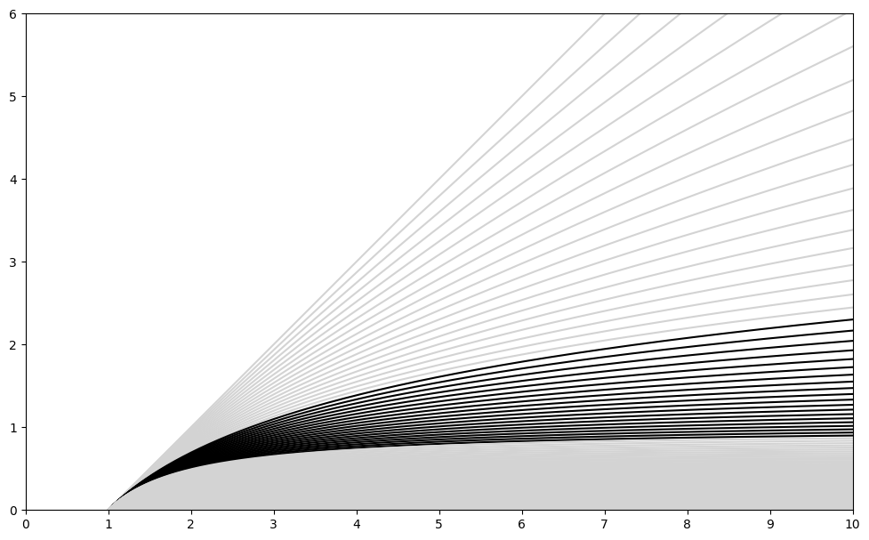
Figure. Plot of the CRRA-utility U(x) for values of α from 0 (top gray line) to ∞ (bottom gray line) in increments of \frac 1{20}. The graphs for a∈[1,2] are shown in black.
Practical values of α are discussed in Mehra & Prescott page 154 and seem to be between one and two. So going forward, the utility function of choice should be
-\frac{1}{x^{α - 1}}
Note. There are many alternative utility functions like CARA, exponential, quadratic, that are mathematically interesting but have little relevance to investment decisions.
http://web.stanford.edu/class/cme241/lecture_slides/UtilityTheoryForRisk.pdf
https://en.wikipedia.org/wiki/Risk_aversion#Relative_risk_aversion
https://en.wikipedia.org/wiki/Hyperbolic_absolute_risk_aversion
https://en.wikipedia.org/wiki/Isoelastic_utility
https://en.wikipedia.org/wiki/Entropic_risk_measure
https://en.wikipedia.org/wiki/Entropic_value_at_risk
https://en.wikipedia.org/wiki/Coherent_risk_measure
Time preference
U(v, t)
Hypothesis: Our risk aversion stays constant over time:
U(v, t) = U_v(v) ⋅ U_t(t) + U_{v0}(v)
https://ocw.mit.edu/courses/economics/14-05-intermediate-macroeconomics-spring-2013/lecture-notes/MIT14_05S13_LecNot_consu.pdf
https://en.wikipedia.org/wiki/Discounted_utility https://en.wikipedia.org/wiki/Time_preference
Sharpe ratio
Define excess return R = \frac{x}{x_0} - R_f with R_f the risk free rate then
S(X) = \frac{\E{R}}{\sqrt{\Var{R}}} = \frac{\E{\frac{X}{x_0} - R_f}}{\sqrt{\Var{\frac{X}{x_0} - R_f}}} = \frac{\frac{\E{X}}{x_0} - R_f}{\sqrt{\frac{1}{x_0^2}\Var{X}}} = \frac{\E{X} - R_f ⋅ x_0}{\sqrt{\Var{X}}}
Suppose a portfolio allocation decision θ is made by maximizing the Sharpe ratio
\argmax_θ S(X(θ))
Under the Von Neumann-Morgenstern theorem we should either be able to find a utility function for this strategy, or find a reason why it is not VNM-rational. To find the Sharpe-ratio utility function U we solve
\argmax_θ S(X(θ)) = \argmax_θ \E{U(X(θ))}
\log S^2 = \log \frac{\p{\E{x} - R_f ⋅ x_0}^2}{\Var{x}} = 2 \log \p{\E{x} - R_f ⋅ x_0} - \log \Var{x}
Equal to quadratic utility U(x) = x - b ⋅ x^2? https://www.d42.com/portfolio/analysis/quadratic-utility
\E{U(x)} = \E{x - b ⋅ x^2} = \E{x} - b ⋅ \E{x^2} = \E{x} - b ⋅ \p{\Var{x} + \E{x}^2}
https://www.princeton.edu/~dixitak/Teaching/EconomicsOfUncertainty/Slides&Notes/Notes02.pdf
https://www.princeton.edu/~dixitak/Teaching/EconomicsOfUncertainty/Slides&Notes/Notes03.pdf
https://en.wikipedia.org/wiki/Sharpe_ratio
https://en.wikipedia.org/wiki/Treynor_ratio
https://en.wikipedia.org/wiki/Information_ratio
Alpha
https://en.wikipedia.org/wiki/Jensen%27s_alpha
References
-
C.E. Shannon (1948). "A Mathematical Theory of Communication" pdf
-
J.L. Kelly (1956). "A New Interpretation of Information Rate" pdf
-
E.O. Thorp (1997). "The Kelly Criterion in Blackjack, Sports Betting, and the Stock Market" pdf
-
R. Mehra & E.C. Prescott (1985). "The Equity Premium: A Puzzle" pdf
-
R. Mehra (2006) "The Equity Premium Puzzle: A Review" pdf
-
A.N. Soklakov (2018). "Economics of Disagreement" arxiv
https://www.earnforex.com/books/en/advanced-forex-trading/The_Sharpe_Ratio.pdf
EXPLAINING THE CHARACTERISTICS OF THE POWER (CRRA)UTILITY FAMILY https://personal.eur.nl/wakker/pdfspubld/08.6powerut.pdf https://doi.org/10.1002/hec.1331
Burr Utility https://www.researchgate.net/publication/46433745_Burr_Utility
Closed Form Solutions in Economics https://papers.ssrn.com/sol3/papers.cfm?abstract_id=2354226 https://poseidon01.ssrn.com/delivery.php?ID=480102116097121106116095076098098030127059060050007025029030118007115009025067002011033056120123040008022109127112095001088105057004042083061118069096073003077009107030077052009069102116081120009068025012083066005100115065008091119015100105102006125013&EXT=pdf&INDEX=TRUE