Fast ζ(2n) calculation
In this post I will show a few very fast algorithms for computing consecutive approximations of $ζ(2n)$, derive my own superior algorithm for high n and produce a hybrid strategy for generating the zeta series required to compute Khinchin’s constant.
In the previous post we posed the following question:
How does one calculate $ζ(2) … ζ(2N)$ fast and accurate up to $B(n)$ bits?
Where:
| Parameter | Value |
|---|---|
| $B$ | 3 321 929 |
| $N$ | $\left\lceil\frac{B}{2}\right\rceil + 1$ |
| $B(n)$ | $B + \left\lceil\log_2 N \right\rceil - \left\lfloor\log_2 n +\log_2 \ln 2 \right\rfloor$ |
There are several interesting algorithms to calculate $ζ(n)$ or the Bernoulli numbers, $B_n$ which are related by:
$$ \zeta(n) = \frac{\vert B_n \vert (2 \pi)^n}{2 n!} $$
-
mpfr_zeta_ui. This is the standard implementation of MPFR, it is accurate up to rounding in the last bit. -
Series summation. This algorithm is trivially summing the $\sum_{[1,\infty)}^k k^{-s}$ terms. However, when s is large the number of terms required to reach the accuracy becomes very low.
-
Euler product. Similar to the summation, but with a product of primes $\prod_{\mathbb{P}}^p \frac{1}{1-p^s}$
-
von Staudt–Clausen algorithm. This is a more involved trick which can produce an exact value of Zeta from an inaccurate one.
-
David Harvey’s BernMM. First calculate $B_n \mathrm{mod}{p}$ for a set of small primes $p$ and then determine an exact value using the Chinese remainder theorem.
The von Staudt-Clausen algorithm
This was our first improvement over mpfr_zeta_ui. In order to get an
exact expression for $ζ$ only the first
$$ 2 + (n+1)(\log_2( n+1 ) - \frac{1}{\ln{2}}) - n \log_2( 2 \pi) $$
bits are required. Unfortunately this number quickly becomes even larger
than the number of bits we require in the final $ζ$ as n grows. However,
for small n it still provides an incredible boost over mpfr_zeta_ui.
Below you can find the source code, the $2 n!$ and $(2\pi)^n$ have been taken out so they can be recycled.
// Table of small primes
extern const uint primes[100000];
// Log2 ( 2 pi )
const double log22pi = 2.6514961294723187980;
// 1 / ln(2)
const double ln2inverse = 1.4426950408889634074;

/// @param zeta is set to ζ(n) - 1
/// @param factor must be set to (2π)^n/(2n!)
/// @returns false when von Staudt-Clausen gives no precision reduction
bool von_Staudt_Clausen_zeta(mpfr_t zeta, uint n, mpfr_t factor)
{
        mp_prec_t low_precision, precision;
        precision = mpfr_get_prec(zeta);
        mpfr_t zeta_low;
        mpfr_t B, term, divisor_sum;
        mpfr_init2(B, precision);
        mpfr_init2(term, precision);
        mpfr_init2(divisor_sum, precision);
        mp_exp_t bits;

        // If n<30 ζ=1 is a good enough apporximation
        if(n < 30)
        {
                low_precision = 2;
                mpfr_init2(zeta_low, low_precision);
                mpfr_set_ui(zeta_low, 1, GMP_RNDN);
        }
        else
        {
                // low_precision = 2 + (n+1)( log2( n+1 ) - 1/ln(2) ) - n log2( 2 pi )
                double lp = 2.0 + (n+1) * ( log2(n+1) - ln2inverse)  - n*log22pi;
                low_precision = floor(lp);
                if(low_precision > precision)
                {
                        return false;
                }
                mpfr_init2(zeta_low, low_precision);
                mpfr_zeta_ui(zeta_low, n, GMP_RNDN);
        }

        // TODO: What is the precision required for B here?
        // B =  zeta / factor   (low precision)
        mpfr_div(B, zeta_low, factor, GMP_RNDN);

        // divisor_sum = Σ 1/p  s.t.  p-1 divides 2n
        mpfr_set_d(divisor_sum, 0.0, GMP_RNDN);
        for(int i=0; true; i++)
        {
                uint prime = primes[i];
                if(prime > n+1)
                {
                        break;
                }
                if(n % (prime-1) == 0)
                {
                        mpfr_set_ui(term, prime, GMP_RNDN);
                        mpfr_ui_div(term, 1, term, GMP_RNDN);
                        mpfr_add(divisor_sum, divisor_sum, term, GMP_RNDN);
                }
        }

        // divisor_sum *= (-1)^(n+1)
        if((n % 4) == 0)
        {
                mpfr_neg(divisor_sum, divisor_sum, GMP_RNDN);
        }

        // von Staudt-Clausen theorem:
        // B = Round( B + divisor_sum ) - divisor_sum
        mpfr_add(B, B, divisor_sum, GMP_RNDN);
        mpfr_round(B, B);
        mpfr_sub(B, B, divisor_sum, GMP_RNDN);

        // zeta = factor * zeta
        mpfr_mul(zeta, factor, B, GMP_RNDN);

        // Remove the term 1
        mpfr_sub_ui(zeta, zeta, 1, GMP_RNDN);

        mpfr_clear(zeta_low);
        mpfr_clear(B);
        mpfr_clear(divisor_sum);
        mpfr_clear(term);
        return true;
}
David Harvey’s multimodular Bernoulli algorithm
Here is the source code and here is the paper paper describing how it works. We do not understand most of it, but the paper is clear about it being the fastest known algorithm for single exact Bernoulli numbers. A zeta function was constructed as follows (again recycling the factors):
/// @param zeta is set to ζ(2n, 2)
/// @param factor must be set to (2π)^n/(2n!)
void multimodular_zeta(mpfr_t zeta, uint n, mpfr_t factor)
{
        mpq_t B;
        mpq_init(B);

        // zeta = |B(n)|
        bern_rat(B, n, 1);
        mpfr_set_q(zeta, B, GMP_RNDN);
        mpq_clear(B);
        mpfr_abs(zeta, zeta, GMP_RNDN);

        // zeta *= factor
        mpfr_mul(zeta, zeta, factor, GMP_RNDN);

        // Remove the term 1
        mpfr_sub_ui(zeta, zeta, 1, GMP_RNDN);
}
Series summation
As said, if we want to beat Harvey’s algorithm we must abuse the fact that we want consecutive inexact values of $ζ$, the series summation lends itself beautifully for that:
$$ \zeta(n) = \sum_{[1,\infty)}^k \frac{1}{k^n} $$
The error introduced when stopping the summation before K is
$$ \sum_{[K,\infty)}^k \frac{1}{k^n} = \zeta(n, K) <\frac{2}{K^n} $$
or expressed in bits of accuracy
$$ B = n\log_2(K) -1 $$
so for B bits of accuracy in the sum we need to add up to but excluding
$$ K = \left\lceil 2^{\frac{B+1}{n}} \right\rceil $$
and these terms on their turn need to be accurate up to
$$ B_{term} = B + \left\lceil \log_2(K) \right\rceil $$
But these terms tend to have a lot of zeros in front of them, in fact, $\left\lfloor n \log_2(k) \right\rfloor$ of them (well, when $k = 2^{m}$ it is off by one, but this doesn’t matter since the remainder will be zero anyway). And since mpfr is a floating point library, these leading zeros do not requite additional precision and can be deducted:
$$ B_{term} = B + \left\lceil \log_2(K) \right\rceil - \left\lfloor n \log_2(k) \right\rfloor $$
/// Fast zeta calculation when few terms are required
/// @param zeta is set to ζ(n) - 1
void series_summation_zeta(mpfr_t zeta, uint n)
{
        // TODO: Discount the zeros of zeta itself
        // TODO: Why do I need to add the extra bit to B?
        mp_prec_t B = mpfr_get_prec(zeta) + 1;

        // K = ⌈ 2^((B+1)/n) ⌉
        uint K = ceil( pow(2.0, (B + 1.0) / n) );

        // B_S = B + ⌈ log2( K ) ⌉
        mp_prec_t B_S = B + ceil(log2(K));
        mpfr_set_prec(zeta, B_S);

        // zeta = 1/2^n
        mpfr_set_d(zeta, 1.0, GMP_RNDN);
        mpfr_div_2ui(zeta, zeta, n, GMP_RNDN);

        mpfr_t term;
        mpfr_init2(term, 2);
        for(uint k=3; k < K; k++)
        {
                // B_term = B + ⌈ log2( K ) ⌉ - ⌊ n log2( k ) - 1 ⌋
                mp_prec_t B_term = B_S - floor( n*log2(k) );
                mpfr_set_prec(term, B_term);

                // term = 1 / k^n
                mpfr_ui_pow_ui(term, k, n, GMP_RNDN);
                mpfr_ui_div(term, 1, term, GMP_RNDN);

                // zeta += term
                mpfr_add(zeta, zeta, term, GMP_RNDN);
        }

        mpfr_prec_round(zeta, B, GMP_RNDN);
        mpfr_clear(term);
}
Powtable series summation
Analysis of the series summation program showed that almost all of the
time was spent in mpfr_ui_pow_ui. We can eliminate this call by
recycling the $\frac{1}{k^n}$ values!
/// Fast zeta calculation when few terms are required
/// @param zeta is set to ζ(n)-1
/// @param powtable is initialized to powtable[k-3] = k^(-2n+2)
/// it will be updated for ζ(n+2)-1 in the process
void powtable_summation_zeta(mpfr_t zeta, uint n, mpfr_t* powtable)
{
        mp_prec_t B = mpfr_get_prec(zeta) + 1;

        // K = ⌈ 2^((B+1)/n) ⌉
        uint K = ceil( pow(2.0, (B + 1.0) / n) );

        // B_S = B + ⌈ log2( K ) ⌉
        mp_prec_t B_S = B + ceil(log2(K));
        mpfr_set_prec(zeta, B_S);

        // zeta = 1/2^n
        mpfr_set_d(zeta, 1.0, GMP_RNDN);
        mpfr_div_2ui(zeta, zeta, n, GMP_RNDN);

        for(uint k=3; k < K; k++)
        {
                // B_term = B + ⌈ log2( K ) ⌉ - ⌊ n log2( k ) - 1 ⌋
                mp_prec_t B_term = B_S - floor( n*log2(k) );
                mpfr_prec_round(powtable[k-3], B_term, GMP_RNDN);

                // powtable[k-3] /= k*k
                mpfr_div_ui(powtable[k-3], powtable[k-3], k*k, GMP_RNDN);

                // zeta += powtable[k-3]
                mpfr_add(zeta, zeta, powtable[k-3], GMP_RNDN);
        }

        mpfr_prec_round(zeta, B, GMP_RNDN);
}

/// Produce a table for powtable_summation_zeta
mpfr_t* init_powtable(mp_prec_t B, uint n)
{
        cout << "Calculating series power table…   0%" << flush;
        timespec start, finish;
        clockid_t cpuclock;
        clock_getcpuclockid(0, &cpuclock);
        clock_gettime(cpuclock, &start);

        B++;

        // K = ⌈ 2^((B+1)/n) ⌉
        uint K = ceil( pow(2.0, (B + 1.0) / n) );
        mpfr_t* powtable = new mpfr_t[K-2];

        // B_S = B + ⌈ log2( K ) ⌉
        mp_prec_t B_S = B + ceil(log2(K));

        for(uint k=3; k < K; k++)
        {
                // B_term = B + ⌈ log2( K ) ⌉ - ⌊ n log2( k ) - 1 ⌋
                mp_prec_t B_term = B_S - floor( n*log2(k) );
                mpfr_init2(powtable[k-3], B_term);

                // powtable[k-3] = 1/k^(n-2)
                mpfr_ui_pow_ui(powtable[k-3], k, n-2, GMP_RNDN);
                mpfr_ui_div(powtable[k-3], 1, powtable[k-3], GMP_RNDN);

                // Display a nice progress indicator
                if(k % 10 == 0)
                {
                        double complete = 100.0 * sqrt(k) / sqrt(K);
                        cout << "\b\b\b" << setw(2) << setprecision(0) << floor(complete) << "%" << flush;
                }
        }
        clock_gettime(cpuclock, &finish);
        cout << "\b\b\b\b100% (in " << timems(start, finish) << " ms)" <<  endl;
        cout << fixed << setprecision(4);

        return powtable;
}
Benchmarking
To decide which algorithms we will use in our attempt to compute $K_0$ we measured (for $B$ = 34, 340 and 3400 kilobit) the run time of:
| Line | Method |
|---|---|
| Red line | mpfr_zeta_ui |
| Blue line | mpfr_zeta_ui with our von Staudt-Clausen implementation |
| Purple line | Darvid Harvey’s bernoulli |
| Green line | Series summation without recycling |
| Black line | Series summation with recycling |
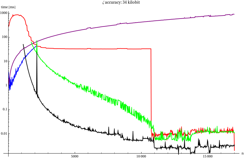
The sudden drop at $n =11 000$ corresponds to the moment when $ζ(2n)-1$ can
be approximated by $2^{-2n}$, apparently that optimisation is included in
mpfr_zeta_ui. At this point the powtable is slightly faster since it
doesn’t allocate memory for an (at this point unnecessary) temporary
variable. The noise corresponds to me using my desktop for other things,
like a screensaver which I forgot to disable, while running the
benchmark.
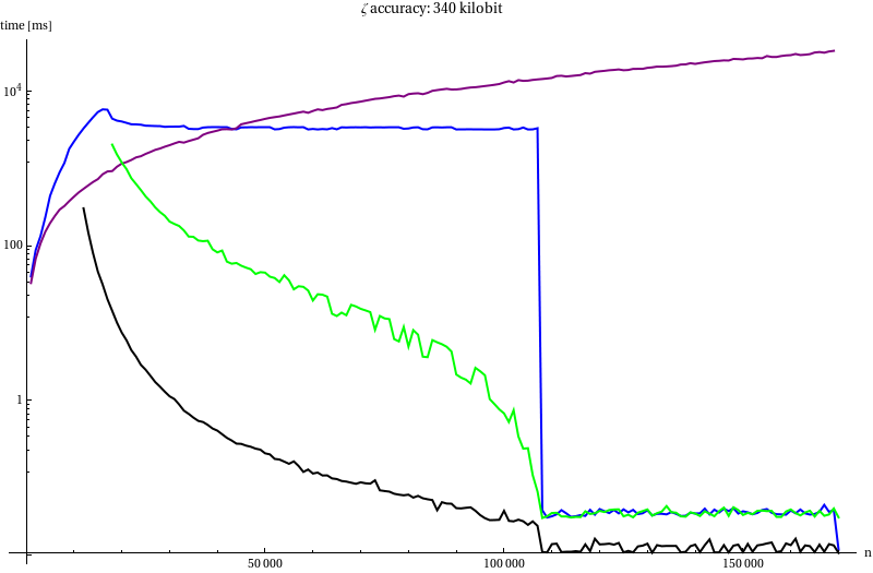
Plain mpfr_zeta_ui was excluded because it would have taken minutes to
compute a single zeta for low $n$. It would have been identical to the
blue line after the peak in the blue line.
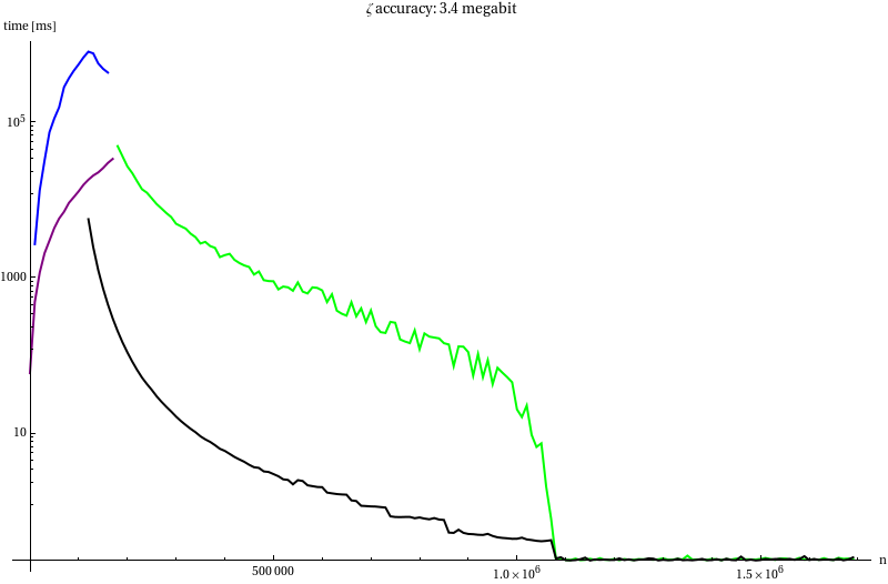
This time the von Staudt-Clausen and Harvey’s method where stopped early since they took up too much time and were not that interesting.
Conclusion
The the mpfr_zeta_ui was not very impressive but with von
Staudt-Clausen it was very good until $n$ grows large. But Harvey’s
method is faster when many bits are required.
Harvey’s algorithm performs very good but is beaten by the series summation when the number of terms included required for the series drops to around a couple hundred.
But the powtable series blows everything away! We will use the powtable series as soon as the number of terms drops below ten thousand, by then its more then three times faster than Harvey’s algorithm and the algorithm kept getting faster as less terms were needed (unlike the Harvey’s, which gets slower for higher $n*$).
There is a reason we don’t start using the powtable method earlier. When $n$ is small exponentially more terms in the table are required, and generating more table items will soon cost more than the time gained by switching to the powtable method a little earlier. Taking 10 000 items seems to be near the optimum, here is how much time it takes to compute the table:
| Accuracy | $n <$ | time |
|---|---|---|
| 34 kb | 1 113 | 1 665 ms |
| 340 kb | 11 121 | 59 298 ms |
| 3 400 kb | 111 201 | 1 667 349 ms |
Integrating the minimum of the running time algorithms reveals that the total time to calculate the $ζ(2n)$'s required for a million decimals of $K₀$ is 9.7 days. Quite long, but not impossible. Calculating a hundred thousand decimal should take about an hour, let’s try that first.